ML and NLP interview questions
Machine Learning Questions
1. Difference between SGD / AdaGrad / Adam / AdamW?
- SGD: \(W_{t+1}=W_t-\lambda \nabla_w J(w)\)
- AdaGrad: \(W_{t+1}=W_t-\frac{\lambda}{\sqrt{G_t+\epsilon}} \nabla_w J(w)\)
- RMSprop: \(W_{t+1}=W_t-\frac{\lambda}{\sqrt{E\left[G^2\right]_t+\epsilon}} \nabla_w J(w)\)
- Adam:
\begin{aligned} & m_t=\beta_1 m_{t-1}+\left(1-\beta_1\right) \nabla_w J(w) \\ & v_t=\beta_2 v_{t-1}+\left(1-\beta_2\right)\left(\nabla_w J(w)\right)^2 \\ & \hat{m}_t=\frac{m_t}{1-\beta_1^1} \\ & \hat{v}_t=\frac{v_t}{1-\beta_2^l} \\ & W_{t+1}=W_t-\frac{\lambda}{\sqrt{v_t}+\epsilon} \hat{m}_t \end{aligned}
- AdamW: \(W_{t+1}=W_t-\lambda (\frac{\hat{m}_t}{\sqrt{\hat{v}_t}+\epsilon}+\alpha W_t )\)
[resource]: a good blog
2. Bias-Variance Tradeoff
Bias is how far off the model’s predictions are from the actual values. Variance is how much the model’s predictions change when trained on different datasets.
- Increasing model complexity decreases bias but increases variance.
- Simpler models have higher bias but lower variance.
3. Overfitting and Underfitting
How to Prevent Overfitting:
- Reduce model complexity : prune decision trees, reduce layers in deep learning.
- Regularization: L1 (Lasso)/L2 (Ridge) regularization, dropout in neural networks.
- Use more training data to help the model generalize better.
- Cross-validation: k-fold CV to test model robustness.
- Early stopping: stop training when validation loss increases.
How to Prevent Underfitting:
- Increase model complexity: use deeper networks, more features.
- Reduce regularization: decrease L1/L2 penalties.
- Use better feature engineering.
- Train for longer.
4. Random Forest vs. Gradient Boosting
Both Random Forest and Gradient Boosting are ensemble learning methods based on decision trees.
| Feature | Random Forest (RF) | Gradient Boosting (GB) |
|---|---|---|
| Training | Parallel (independent trees) | Sequential (each tree fixes previous errors) |
| Bias vs. Variance | Higher bias, lower variance | Higher variance, lower bias |
| Overfitting | Less prone to overfitting | Can overfit if not tuned properly |
| Speed | Faster (parallel computation) | Slower (sequential computation) |
| Best For | General-purpose models, stability | High-performance tasks, structured data |
| Robustness | Works well with default settings | Requires careful tuning |
5. Decision tree for classification
The goal is to measure impurity. Two metrics:
- Gini Impurity: For each node, calculate \(Gini=1-\sum_{i=1}^C p_i^2\). \(C\) is the number of classes, \(p_i\) is the proportion of samples belonging to class \(i\) in a given node. 0 means the node is pure. Higher values mean more class mixing.
- Entropy and Information Gain: \(Entropy =-\sum_{i=1}^C p_i \log _2 p_i\). Entropy measures how "uncertain" or "mixed" the class labels are in a node. Lower entropy means the node is more "pure". \(I G= Entropy_{p a r e n t}-\sum\left(\frac{N_i}{N} \times\right.\) Entropy \(\left._i\right)\)
6. Bootstrap
Bootstrap is a data resampling technique used to create multiple datasets from a single dataset by randomly sampling with replacement. It is commonly used in ensemble learning (like Random Forest) to improve model stability and performance.
Advantages of Bootstrap:
- Reduces variance by averaging multiple models.
- Improves generalization by training on diverse datasets.
- Works well for small datasets where splitting into train/test might lose valuable data.
7. L1 and L2 regularization
L1 Regularization (Lasso):
- Encourages sparsity (sets some weights to exactly zero).
- Leads to feature selection (removes less important features).
L2 Regularization (Ridge)
- Shrinks weights toward zero but does not eliminate them.
- Helps with multicollinearity (reduces variance but keeps all features).
7. Explain Principal Component Analysis (PCA)
Steps:
- Standardize the Data: Each feature has mean = 0 and variance = 1.
- Compute the Covariance Matrix: Measures the relationships between features.
- Compute Eigenvalues & Eigenvectors
- Select the Top Principal Components
- Project Data onto New Axes
9. PCA vs LDA
PCA (Principal Component Analysis) and LDA (Linear Discriminant Analysis) are both dimensionality reduction techniques. PCA: Focuses on preserving variance in the data. LDA focuses on maximizing class separability.
Why PCA focuses on the variance of data?
"variance in the data" means how spread out the data points are across different dimensions. Variance measures how much the values in a dataset differ from the mean. If a feature has high variance, it means the values are more spread out, which typically indicates it holds more distinguishing information. PCA finds the directions having the highest variance because these directions contain the most information.
| Feature | PCA (Principal Component Analysis) | LDA (Linear Discriminant Analysis) |
|---|---|---|
| Purpose | Maximizes variance to retain the most information | Maximizes class separability for better classification |
| Supervision | Unsupervised (does not use class labels) | Supervised (requires class labels) |
| What It Finds | Directions with the highest data variance | Directions that best separate different classes |
| How It Works | Computes eigenvectors of the covariance matrix | Computes eigenvectors of the scatter matrices (between-class and within-class) |
| Dimensionality Constraint | Can reduce dimensions up to the number of original features | Can reduce dimensions to at most C - 1 (where C = number of classes) |
| Best For | Data compression, feature reduction, visualization | Classification tasks where class separation is important |
| Output | Orthogonal principal components capturing the most variance | New axes optimized for class distinction |
8. Batch Normalization and Layer Normalization
Batch Normalization normalizes neuron outputs across the batch dimension for each feature, but layer normalization across the feature dimension for each individual input sample.
| Feature | Batch Normalization | Layer Normalization |
|---|---|---|
| Normalization Axis | Across batch (for each feature) | Across features (for each sample) |
| Dependency | Depends on batch size | Works independently of batch size |
| Use Case | CNNs, large batch training | RNNs, Transformers, small batch training |
| Training Stability | Can be unstable in small batches | Stable for all batch sizes |
Use BN when working with structured grid-like data. Use LN when working with sequential or non-grid data.
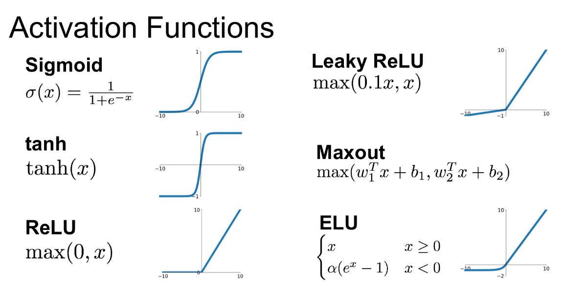
10. Activation Functions
- ReLU: \(f(x)=\max (0, x)\)
- Leaky ReLU: \(f(x) = \max(0.01x, x)\)
- Sigmoid: \(f(x) = \frac{1}{1 + e^{-x}}\)
- Tanh: \(f(x) = \frac{e^x - e^{-x}}{e^x + e^{-x}}\)
- Softmax: \(f(x_i) = \frac{e^{x_i}}{\sum_{j} e^{x_j}}\)
Why is ReLU better and more often used than Sigmoid in Neural Networks?
1. Avoids the Vanishing Gradient Problem: the derivative of the sigmoid function is very small when 𝑥 is large or small
2. Computational Efficiency: Simple max(0, x) operation, which is much faster to compute exponentials.
11. Describe how convolution works
key concepts: convolution, kernel, stride, receptive field.
receptive field: refers to the region of the input image that a neuron in a particular layer "sees". As we go deeper in the network, receptive fields grow larger, capturing broader and more complex features. By the final layers, neurons can "see" almost the entire image. \(RF = RF_{pre} + (K-1) \times S\).
12. Why do we use convolutions for images rather than just FC layers
- Preserve Spatial Structure: Images have local patterns (e.g., edges, textures), and convolutions capture them while FC layers lose spatial relationships.
- Reduce Parameters: A fully connected layer requires each neuron to connect to every pixel, leading to huge parameter sizes for high-resolution images.
- Translation Invariance: Convolutions allow the network to detect patterns anywhere in the image, while FC layers memorize specific positions.
13. Implement a sparse matrix class
14. Reverse a bitstring
data = b'\xAD\xDE\xDE\xC0'
my_data = bytearray(data)
my_data.reverse()
15. What is the significance of Residual Networks
The main thing that residual connections did was allow for direct feature access from previous layers. This makes information propagation throughout the network much easier. Also, it helps to solve the problem of vanishing gradients.
16. How to deal with imbalanced dataset?
- Oversampling or undersampling
- Data augmentation
- Algorithm-wise: Class Weight Adjustment,
- Using appropriate metrics: e.g. Precision, Recall, F1-score, AUC-ROC Curve
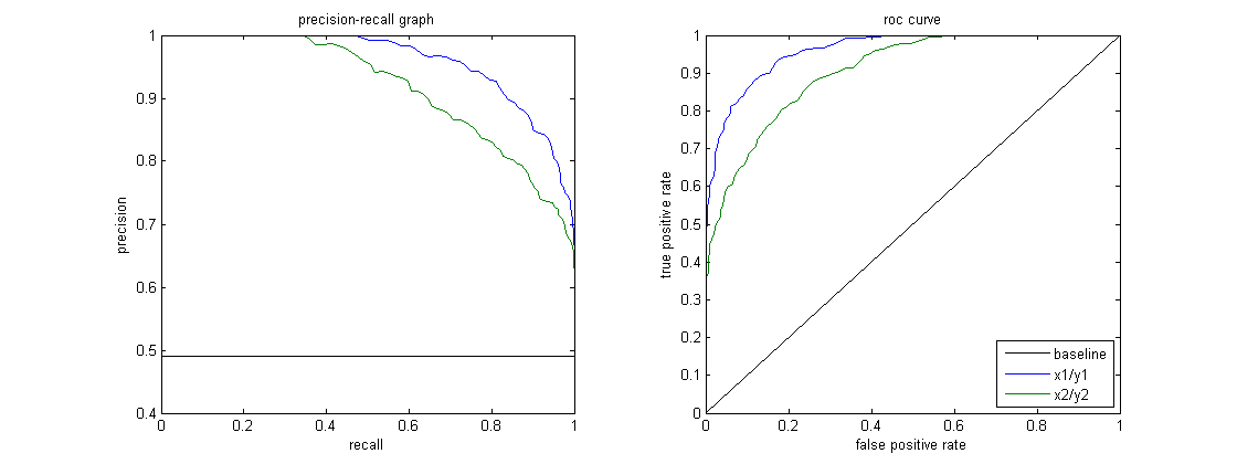
17. Precision, Recall, F1-score, AUC-ROC Curve, P-R Curve
- Precision: How many predicted positives were actually positive? \(Precision = \frac{TP}{TP+FP}\)
- Recall: How many actual positives did we catch? \(Recall = \frac{TP}{TP+FN}\)
- ROC Curve: True Positive Rate (TPR, Recall) [y-axis] is how many of the actual positives did we catch. False Positive Rate (FPR) [x-axis] is how many of the actual negatives did we incorrectly label as positive? \(TPR = \frac{TP}{TP+FN}\); \(FPR = \frac{FP}{FP+TN}\).
- AUC: Area Under the ROC Curve
ROC Curve shows model performance at various thresholds.
P-R Curve: Precision (Positive Predictive Value) [y-axis], Recall (Sensitivity) [x-axis]
| Scenario | Use ROC Curve? | Use P-R Curve? |
|---|---|---|
| Balanced dataset | ✅ Yes | ❌ No |
| Imbalanced dataset (rare positives) | ❌ No | ✅ Yes |
| False Positives matter more | ❌ No | ✅ Yes |
| Overall classification performance | ✅ Yes | ❌ No |
| Detecting rare events (e.g., fraud, disease) | ❌ No | ✅ Yes |
18. Difference between supervised, unsupervised, and reinforcement learning.
| Type | Supervised Learning | Unsupervised Learning | Reinforcement Learning |
|---|---|---|---|
| Definition | Learns from labeled data (input-output pairs) | Learns patterns from unlabeled data | Learns by interacting with an environment and receiving rewards |
| Data Type | Labeled (e.g., (image, label)) | Unlabeled (only input data) | Sequential decision-making data |
| Goal | Minimize error between predictions and true labels | Find hidden structures/patterns | Maximize cumulative rewards |
| Examples | Classification (e.g., spam detection), Regression (e.g., house price prediction) | Clustering (e.g., customer segmentation), Dimensionality Reduction (e.g., PCA) | Game playing (AlphaGo), Robotics, Self-driving cars |
| Training Approach | Uses loss function (e.g., MSE, Cross-Entropy) | Finds similarities or distributions | Uses trial-and-error learning (policy optimization) |
19. Techniques for data augmentation in CV.
- Geometric Transformations: Rotation, Flipping, Scaling
- Color-Based Augmentations: Brightness Adjustment, Contrast Adjustment, Hue & Saturation Changes
- Noise-Based Augmentations: Gaussian Noise, Blur, Cutout
20. What is vanishing gradient?
Vanishing gradient problem occurs in deep neural networks when gradients become extremely small during backpropagation, making it difficult for the network to learn.
Why Does It Happen?
- Activation Function Effects: such as Sigmoid and Tanh functions
- Weight Initialization Issues: such as weights are too small
- Deep Networks (Many Layers): If each derivative is a small number (e.g., <1), their product shrinks exponentially as we go deeper, leading to almost zero gradients for early layers.
How to address vanishing gradient?
- Use ReLU Instead of Sigmoid or Tanh
- Batch Normalization
- Better Weight Initialization
- Use Residual Networks (ResNet)
21. How to deal with exploding gradient?
- Gradient Clipping: Set a threshold to clip gradients during backpropagation.
- Use Smaller Learning Rate: Reducing the learning rate prevents drastic weight updates.
- Weight Regularization
- Use Proper Weight Initialization
- Use Normalization
- Switch to a Different Activation Function: ReLU (instead of sigmoid/tanh) helps mitigate vanishing gradients but can cause exploding gradients. Try LeakyReLU or ELU instead.
22. What are dropouts?
During each forward pass, dropout randomly "drops" (sets to zero) a percentage of neurons in the layer. This prevents the network from becoming too dependent on specific neurons and forces it to learn more robust and generalizable features.
23. How does t-SNE work?
t-SNE visualizes high-dimensional data by placing similar points close together in a 2D or 3D space.
24. Direct Preference Optimization(DPO)
Direct Preference Optimization (DPO) is a training method for aligning language models (LLMs) with human preferences without needing reinforcement learning. It serves as an alternative to Reinforcement Learning from Human Feedback (RLHF) while maintaining simplicity and efficiency.
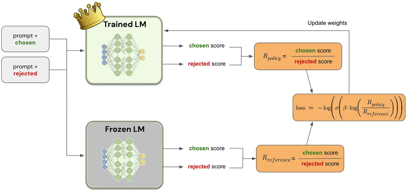
At the very beginning, the initial loss should be close to zero. \( Loss = \log \frac{P_\theta\left(y_{\text {preferred }} \mid x\right)}{P_\theta\left(y_{\text {disliked }} \mid x\right)}-\log \frac{P_{\text {ref }}\left(y_{\text {preferred }} \mid x\right)}{P_{\text {ref }}\left(y_{\text {disliked }} \mid x\right)}\)
Even though the initial loss is near zero, training gradually adjusts \(P_\theta\) to diverge from \(P_{\text {ref }}\) and increase preference alignment. Though the loss starts at zero, gradient updates still occur. The model slightly shifts probabilities toward the preferred responses.
25. DPO vs RLHF
| Feature | DPO (Direct Preference Optimization) | RLHF (Reinforcement Learning from Human Feedback) |
|---|---|---|
| Training Complexity | Simple (direct fine-tuning) | Complex (requires multiple stages: reward model + RL) |
| Optimization Method | Supervised learning (log-ratio loss) | Reinforcement learning (PPO, policy optimization) |
| Reward Model Needed? | ❌ No | ✅ Yes (trained separately using preference data) |
| Loss Function | Log-ratio of preference probabilities | Reward function trained via RL (KL-regularized PPO) |
| KL Regularization | Implicitly baked into the objective | Explicit KL penalty required to prevent divergence |
| Gradient Stability | More stable (direct loss minimization) | Unstable (gradient explosion, KL tuning required) |
| Computational Cost | Lower (direct preference fine-tuning) | Higher (training a reward model + RL updates) |
| Convergence Speed | Faster | Slower |
| Interpretability | More interpretable (directly optimizes preference scores) | Less interpretable (reward models can introduce bias) |
| Primary Use Cases | Aligning LLMs with human preferences (e.g., chatbots, summarization) | Preference alignment, reinforcement learning tasks (e.g., AI safety, robotics) |
| Challenges | Still under research, requires careful hyperparameter tuning | Instability, difficulty in fine-tuning rewards |
26. Difference between Discriminative models and Generative models
| Feature | Discriminative Models | Generative Models |
|---|---|---|
| Definition | Learn the decision boundary between classes | Model the actual distribution of the data |
| Probability Modeled | \(P(y \| X)\) (Conditional probability of labels given input) | \(P(X, y)\) (Joint probability of input and labels) |
| Goal | Directly classify or predict labels | Generate new data or classify by computing likelihood |
| Examples | Logistic Regression, SVM, Random Forest, Neural Networks | Naïve Bayes, Gaussian Mixture Model (GMM), GANs |
| Advantage | Usually more accurate for classification tasks | Useful for data generation and handling missing data |
| Disadvantage | Requires large labeled datasets, less flexible for missing data | Can be computationally expensive and harder to optimize |
In short:
- Discriminative models focus on learning boundaries for classification.
- Generative models learn the data distribution and can generate new samples.
NLP
1. Transformers and Multi-head Self-attention
Please see the code: https://github.com/audreycs/transformer_from_scratch.
1. Why using multi-head?
A: Multiple attention heads allow the model to learn different aspects of the input simultaneously.

2. When calculating Multi-Head Attention, why use scaling before taking the softmax?
A: To stabilize gradients and improve numerical stability. Softmax() makes the value more polarized: large values get larger in magnitude after softmax, and small values get smaller -> this causes gradients more unstable.

3. why adding positional encoding in the input?
A: Transformers have no recurrence (RNNs) or convolution (CNNs), meaning they do not
inherently understand token order. Unlike RNNs, which process sequences sequentially,
Transformers process all tokens in parallel, making them faster but order-agnostic.
Add Positional Encoding (PE) to the input embeddings so that the model can capture token
positions and sequence order.
2. Absolute Position Encoding
Transformer's absolute PE is added to token embeddings:
The limitation of absolute PE:
The dot product between two positional encodings depends only on the absolute value of the
index difference between the two positions, and therefore cannot represent directional information.
When the input embeddings are fed into the attention mechanism, this can lead to ambiguous
recognition of distances, meaning the ability to represent relative positions through positional
encoding can be disrupted by matrix projections.

As a result, later improvements in BERT adopted learnable positional encodings, and it is
updated during training.
3. What is RoPE? Why is it needed? When and where does it be applied?
RoPE (Rotary Positional Embedding) encodes token positions by rotating the query/key vectors in attention (in 2D pairs), so attention scores depend on relative position.
Self-attention alone is order-agnostic. RoPE injects position information in a way that naturally supports relative-distance awareness and works well for long-context behavior.
In each attention layer: after computing Q and K (and usually after splitting into heads), apply RoPE to Q and K before computing attention scores. It’s used in both self-attention and causal/masked self-attention; the mask is applied afterward.
Use either RoPE during attentin calculation or Positional Encoding during input, not both.
4. What is KV Cache?
KV cache (Key–Value cache) is a speed-up trick used during autoregressive decoding in transformer LLMs.
- In each attention layer, every generated token produces a Key (K) and a Value (V).
- Instead of recomputing K/V for all previous tokens every time you generate the next token, the model stores past K/V in memory.
- When generating token t+1, it only computes K/V for the new token and attends to the cached past K/V.
When generating a new token, only the query of the last token is used (Q[-1]), compute with the K to get the attention, and compute with the V.
KV cache accelerates the attention computation during decoding (inference). Only K and V need to be store, Q doesn't need because each inference only needs the query embedding of the last token.
5. What is Multi-query KV Cache?
Multi-query KV cache (MQA) is an attention variant where all attention heads share the same Keys (K) and Values (V), but each head still has its own Query (Q).
6. What is PagedAttention?
PagedAttention is vLLM’s attention method that works with a paged / block-based KV cache.
Instead of assuming all past K/V for a sequence live in one contiguous chunk of GPU memory, vLLM stores KV in many fixed-size blocks (“pages”). Each sequence keeps a page table (indirection map) that tells the model where its KV blocks are physically stored.
PagedAttention has better usage of the memory.
7. Layer Norm vs. RMSNorm
Compared to Layer Norm, RMS Norm removes the part of subtracting the mean during calculation, with the idea of treating the mean as 0, leading to faster computational speed and almost the same performance.
8. What parameters are learnable in Transformer?
- Token Embeddings
- For each attention layer: four weight matrix \(W_Q\), \(W_K\), \(W_V\), and \(W_o\).
- Layer Norm/RMSNorm: learnable scale and shift
- FFN network
- Decoding head
9. What's the order of applying norm, RoPE, and residual connection? What's the difference between Pre-norm and Post-norm?
Typical (modern LLM / Pre-norm) order:
- Norm → QKV projections → RoPE on Q & K → Attention/MLP → Residual add
Post-norm (classic Transformer) order:
- Sublayer (QKV→RoPE→Attn or MLP) → Residual add → Norm
Pre-norm vs Post-norm:
- Pre-norm: normalize before each sublayer; usually trains deeper models more stably.
- Post-norm: normalize after residual addition; original design.
10. Model structure of LLMs
The mainstream chat LLMs (GPT / Llama / Qwen / DeepSeek / Gemini) are overwhelmingly decoder-only.
Decoder-only vs. Encoder-Decoder (key difference):
- Decoder-only is trained with next-token prediction. It is natural for text continuation task. Encoder–decoder pretraining is usually framed as sequence-to-sequence. It is great for "transform this input into that output" task.
- Decoder-only is simpler and scales better. Decoder-only models naturally support KV caching
Encoder-decoder is "weird" for chat continuation task, as the generated tokens keeps growing,
but the encoding sequence is "fixed". If re-encoding frequently, it adds overhead and complexity.

Encoder–decoder still has real advantages in some settings:
1. pure transformation tasks (translate, summarize, extract)
2. cases where we encode once and produce multiple outputs
11. Flash attention
FlashAttention proposes an acceleration technique that significantly speeds up computation, saves memory, and achieves IO-aware precise attention. FlashAttention can be applied during both training and inference.
In original attention calculation, the big matrices (Q, K, V) are huge for long sequences, and moving them to/from GPU memory is often the real bottleneck.
FlashAttention never materializes the full attention matrix in GPU high-bandwidth memory. Instead it:
- tiles / blocks the computation (works on small chunks of Q, K, V at a time),
- keeps intermediate data in fast on-chip memory (SRAM/shared memory),
- uses a streaming softmax trick (so you can compute softmax correctly across blocks),
- and writes out only the final output.
Result: much less memory traffic and typically significant speedups, especially as context length grows.
Model Training
1. What is SFT and DPO?
2. Policy-gradient algorithm
REINFORCE vs. Actor–Critic
Understand four models in Actor–Critic:
- actor model
- critic/value model
- reward model
- reference model (optional)
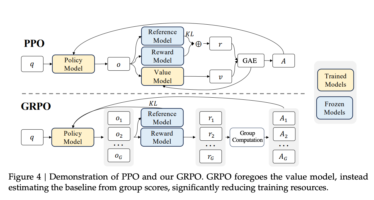
3. What is PPO?
PPO is a specific actor–critic algorithm. It adds a trust-region-like constraint via a clipped objective so updates don’t change the policy too much:
The Critic Model can be initialized in multiple common ways. For example, a value head (typically a linear projection layer) be added on top of LLM to predict scalar values.
Why a critic model is needed in PPO?

If we use only the reward to train the actor model, the updates are very noisy.
The critic model gives a low-noise training signal (variance reduction).
It approximates the expected return so you learn from the surprise:
4. What is RLHF?
RLHF process:
- SFT
- Train a reward model from preference data
- RL fine-tuning the policy with PPO + KL control
5. What is GRPO?
GRPO samples multiple outputs \({O_1, O_2, O_3..., O_G}\) for the same question \(q\), then the Reward model assigns a reward value to each of these outputs, and finally produces an estimate of the advantage function.
GRPO removes the Critic model. Instead of using Critic model to compute the Advantage, GRPO uses the follow formula:
GRPO normalizes the reward within a sampled group and treats it as the advantage value, and assigns this normalized reward to each output tokens. Simply speaking, the reward for the current output is compared to the average reward of all outputs, and the difference between them is the advantage (the value can be positive or negative).
6. What is reward hacking in RL?
Inaccurate or biased reward functions can lead to agents exploiting them in unintended ways, resulting in behavior that does not align with human expectations, or even causes harm—a phenomenon known as reward hacking.
In reward hacking, we often observe that the training reward keeps increasing, but human-evaluated performance drops.
Designing proper reward functions often requires substantial effort from domain experts.
7. Online vs. Offline RL
Online RL: The core idea of Online RL is to let the model generate its own responses, and then we score the quality of those responses to guide model updates.
Offline RL: In contrast, Offline RL does not require the model to generate answers on its own. Instead, it learns from a fixed dataset of collected responses, with associated preference scores.
8. Training data difference between SFT and RL
SFT: We want the model to learn what a good answer looks like, so we need high-quality data.
RL: Teaches the model how to choose among possible answers.
| Aspect | SFT data | RL data |
|---|---|---|
| Data size | Usually smaller can still work well (because every example is a full “gold” target). Adding more helps, but diminishing returns if quality isn’t high. | Often needs more total volume: (1) a large prompt pool to sample from, and (2) a preference set (pairs/rankings). Preference labels are cheaper than writing gold answers, so you can scale to hundreds of thousands to millions of comparisons in big setups. RL rollouts themselves are generated on the fly. |
| Data quality | Extremely high bar. Labels are the exact behavior you imprint. Noise/bad answers directly teach bad habits (style, facts, safety). Consistency in formatting/tone matters a lot. | Quality still matters, but it’s a bit different: you need reliable relative judgments (A better than B) and well-defined criteria. Label noise is more tolerable than in SFT if you have enough data, but systematic bias in preferences (or a flawed reward model) can push the policy in wrong directions (“reward hacking”). Prompt distribution quality is also crucial. |
Other Blogs
-
ML questions 1: https://northern-dracopelta-98c.notion.site/5b22e124e16d4b2d937940367ca20eb0?v=19feabb85e9e4b54bc498579b3c7f1c5
-
ML questions 2: https://github.com/nxpeng9235/MachineLearningFAQ/blob/main/bagu.md
-
MLE Interview Prep 2025: https://occipital-alfalfa-20e.notion.site/MLE-Interview-Prep-2025-2879301bf517804bb515fe9731275166
-
AI Learning: https://comfyai.app/about